Decline in Inverse and Leveraged ETFs

So this post isn’t about programming, but it has a lot of math, and it’s about understanding how something works. Lately my investing has used some ETFs, but I’ve read that if your ETF is inverse or leverage, then it gradually loses money over time—simply because of the mathematics. I wanted to investigate just how this worked.

First, a bit of background: an ETF is an Exchange-Traded Fund, a pretty new thing. It’s not a stock, but a type of derivative used to track something else, such as a sector of stocks. In this regard it’s a bit like an index, but more flexible. So you could have an ETF tracking the performance of pharmaceutical stocks, or financial stocks, or the S&P 500. They are a little different from index-based mutual funds. You can trade them any time during the day, and they don’t have the high minimum purchases required by some mutual funds. On the other hand, you pay a commission, unlike a non-load mutual fund. (In some cases this may not be true.)

But the really interesting thing about them is that they can be leveraged or inverse. A leveraged fund aims to achieve some multiple of the daily change of the underlying index. So while the SPY fund tracks the S&P 500, you can get 2x the S&P 500 (both up and down) with the SSO fund. This greater volatility gives you the potential for more profit with each trade, diminishing the relative size of the commission. It’s a bit like you invested twice as many dollars as you actually have.

An inverse fund is a leveraged fund with a negative multiplier. You can get funds at -1x, -2x, or I think even -3x. This essentially lets you short the market, something difficult for retail investors to manage. Also, unlike with shorting, you don’t risk an unlimited amount of money. You only risk the money you use to buy the ETF.

The fly in the ointment is that ETFs, when leveraged or inverse, gradually decline in value. Let’s say we have an index that start at 100, declines to 80 (-20%), then goes back up to 100 (+25%). Now let’s say we were tracking it with four ETFs, a 1x, a -1x, a 2x, and a -2x. They all start at 40. Here are the results:

Fund	t0	t1	t2
Index	100	80	100
1x ETF	40	32	40
-1x ETF	40	48	36
2x ETF	40	24	36
-2x ETF	40	56	28

As you can see, all our ETFs lost money, except the 1x version. Conspicuously, the -1x and 2x ETF lost the same amount, but the -2x ETF lost more. If we had reversed the order of changes (100 to 125 to 100), we would see the same results.

So I set out to analyze the mathematics behind all this. Let’s start with some equations describing our targeted fund, the index. I’ll call its initial value T. Our intermediate value will be T’. Our final value will be T’‘—but of course this is equal to T. Let’s call the first percent change d, and the second percent change d’. That gives us these equations:

T’ = T + dT T = T’‘ = T’ + d’T’ If we substitute T for T’ and solve for d’, we get: T = (T + dT) + d’(T + dT) 0 = dT + d’(T + dt) -dT / (T + dT) = d’ d’ = -d / (1 + d) Now let’s write out the equations for our derived fund, D (the ETF). We’ll use D, D’, D’‘ to correspond with T, T’, T’‘. The multiplier of our ETF will be f. So in a 1x ETF, f = 1, but in a -2x ETF, f = -2. That gives us these equations: D’ = D + fdD D’‘ = D’ + fd’D’ Substituting, we get: D’‘ = (D + fdD) + f * (-d/(1+d)) * (D + fdD) So far so good, but I’m really interested in the percent lost for each up-and-down cycle. The absolute loss is D - D’‘, so the percent loss is (D - D’‘) / D. Let’s call this L. That gives us: L = (D - D’‘) / D L = (D - ((D + fdD) + f * (-d/(1+d)) * (D + fdD))) / D L = (D - D - fdD - f * (-d/(1+d)) * (D + fdD)) / D L = -fd - f * (-d/(1+d) * (1 + fd) L = fd/(1+d) * (1 + fd) - fd L = fd(1+fd) / (1+d) - fd(1+d) / (1+d) L = (fd(1+fd) - fd(1+d)) / (1+d) L = fd(1+fd-1-d) / (1+d) L = fd(fd-d) / (1+d) L = fd²(f-1) / (1+d) L = f(f-1) * d² / (1+d) That final equation tells us that the loss is proportional to f and d. Well, d is kind of obvious: the more our underlying index changes, the more the ETF will change. But f is quite interesting. The more leveraged we are, the more we lose on each cycle. Although neither factor is as simple to write out as we might like, consider this. f(f-1) is almost f*f, or f²: f*(f-1) < f*f f*(f-1) < f² The effect of f is almost a square. We could imagine this as f^1.9, although that isn’t quite right.

At first glance, it seems we could make a similar simplification with d, since d²/(d+1) is a little less than d²/d:

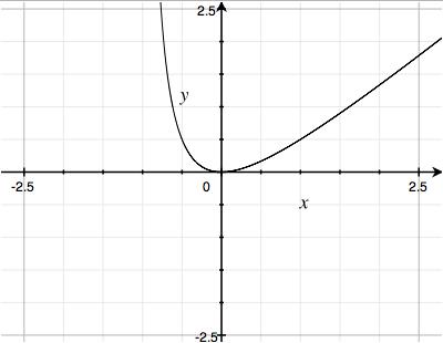
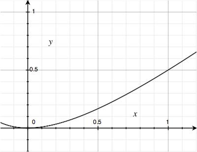
d²/(d+1) < d²/d d²/(d+1) < d So d’s effect would be a little less than d: sort of like d^0.9. But this is misleading, because d²/(d+1) only approximates d for large values, and our d will (probably) never go above 1. In fact it’s only interesting for values like 0.01 or 0.1 or maybe (gulp) 0.5. At that range, we get values like:

d	d2/(d+1)
0.01	0.00009
0.02	0.00039
0.03	0.00087
0.04	0.00153
0.05	0.00238
0.10	0.00909
0.20	0.03333
0.30	0.06923
0.40	0.11428
0.50	0.16666

The graph looks like this:

Or at close range, like this:

All this means that comparatively speaking, f has a greater effect than d.

We could chart f’s effect for different levels of leverage:

f	f(f-1)
1	0
2	2
3	6
4	12
5	20
6	30
-1	2
-2	6
-3	12
-4	20
-5	30

In other words, each “step” up in leverage increases your loss, and going inverse counts as one additional “step.”

By multiplying these values with those from d’s table, you can see your loss for each cycle. For a 2x or -1x ETF, you lose about 2% of your investment for each 10% cycle, or 0.02% for each 1% cycle. For a -2x ETF, you lose about 6% for a 10% cycle or 0.06% for a 1% cycle. Best not to stay in these investments for too long!

The next question is: how long is right? I guess you could look at the last few years to count the number of cycles, and try to figure out an ETF’s theoretical decline if the market had no net change. But the conventional wisdom answer seems to be about a week, and this sounds right to me. You’re really betting on the direction of the next move, and if you get that wrong, it’s going to cost you. So to make money with these ETFs, you need to get not just the direction right, but the timing, too. It’s hard enough just to get the direction! This need to be right about timing makes them risky for the same reason options are risky: your bet only has so long to play out.

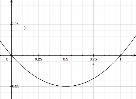
Now here is another thought. Take a look at a graph of f(f-1):

As you can see, between 0 and 1, this graph dips below 0. That means that if you had a x0.5 ETF, say, you would actually make money over time. I wonder if there are practical reasons to prevent this, or if the return is just too small, so you’d do better putting your money in a bank. Anyway, it’s an interesting thought… .

blog comments powered by Disqus Prev: Sorting Out the Confusion: 32- vs. 64-Bit, CLR vs. Native, C# vs. C++ Next: Variation on C Password Dictionary Variator